3D Audio Visualizers

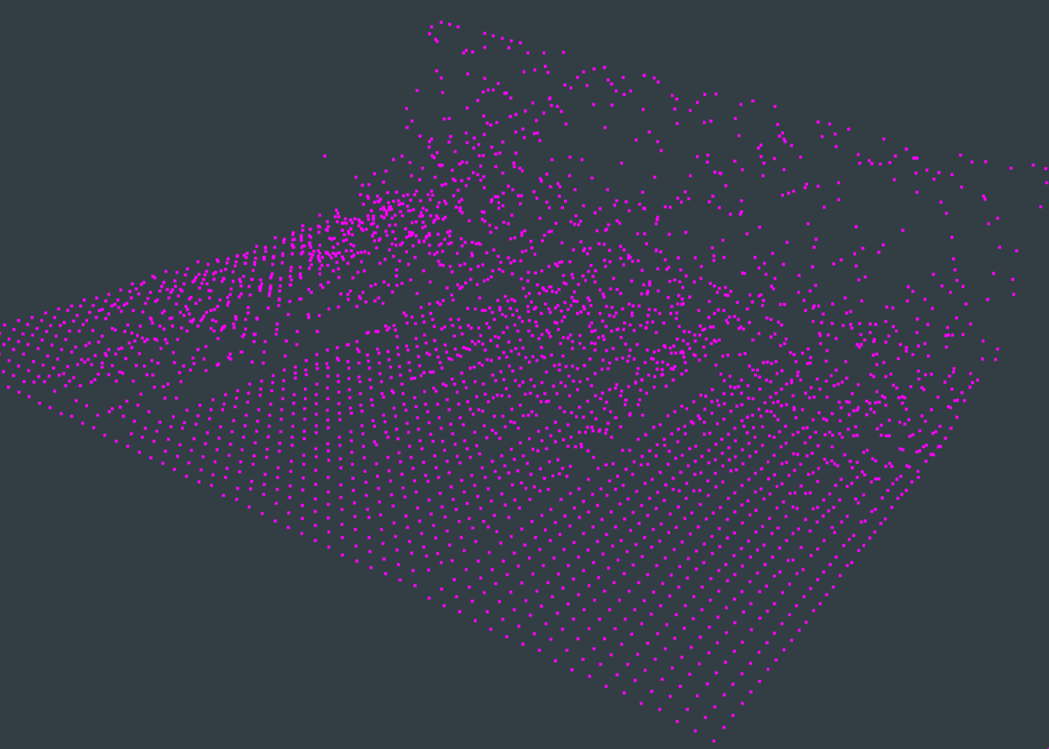
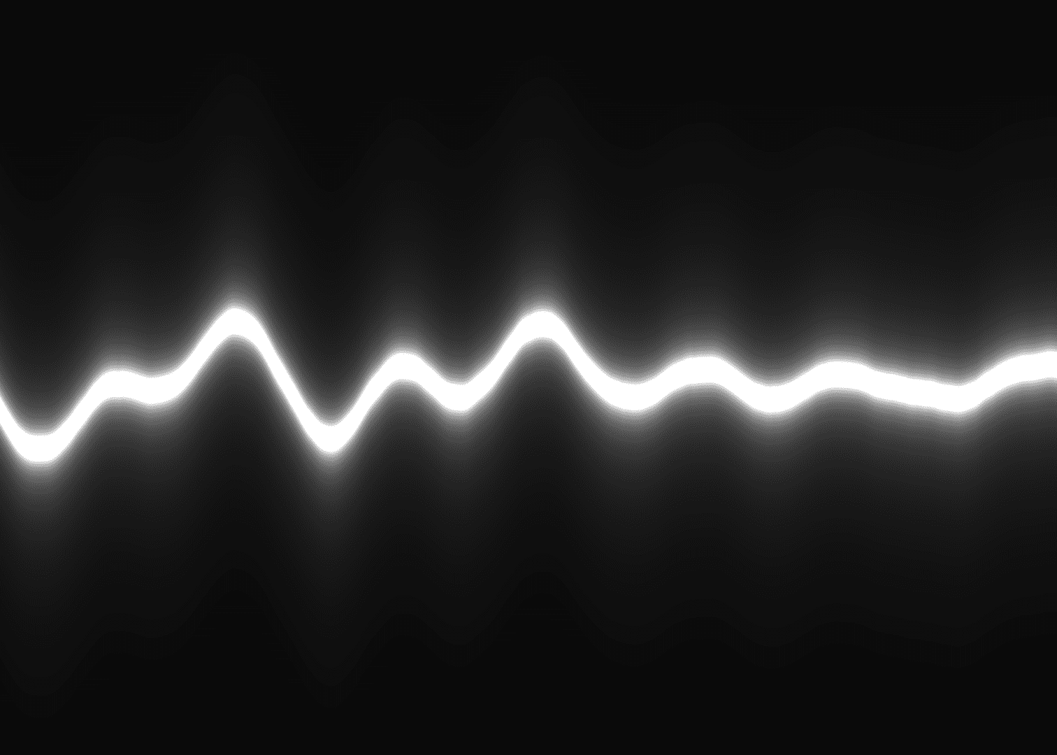
A 3D audio visualizer app I created in 2017 for Computer Graphics class at university. It contains 3 audio visualizers including a 2D oscilloscope, 3D oscilloscope pipe, and a 3D frequency spectrum. The app takes audio input from a microphone or audio file and visualizes it in realtime, allowing rotation of the 3D visualizers by dragging with a mouse. I created the app (as shown in the YouTube video) in a single week using OpenGL shaders, JUCE, and C++.

#Things I Learned

• Ring Buffers are important to realtime, lock-free programming (especially for audio development). The realtime audio thread can quickly feed audio into the ring buffer repeatedly without any real performance hit. Other “not as realtime” threads, such as the graphics thread can pull from that ring buffer, to grab the most recent data. These lower priority threads can allow for some latency in their callbacks. For example, if you drop a few visual frames in your graphics thread, no one will really notice. But, if you drop some samples in your audio thread, the audio will sound bad and crackle. This video by Timur Doumler was very informative.
• OpenGL and shaders can be complex to setup, but they are very powerful and modular once you know how to use them. LearnOpenGL.com was a great resource for learning how to use OpenGL shaders.
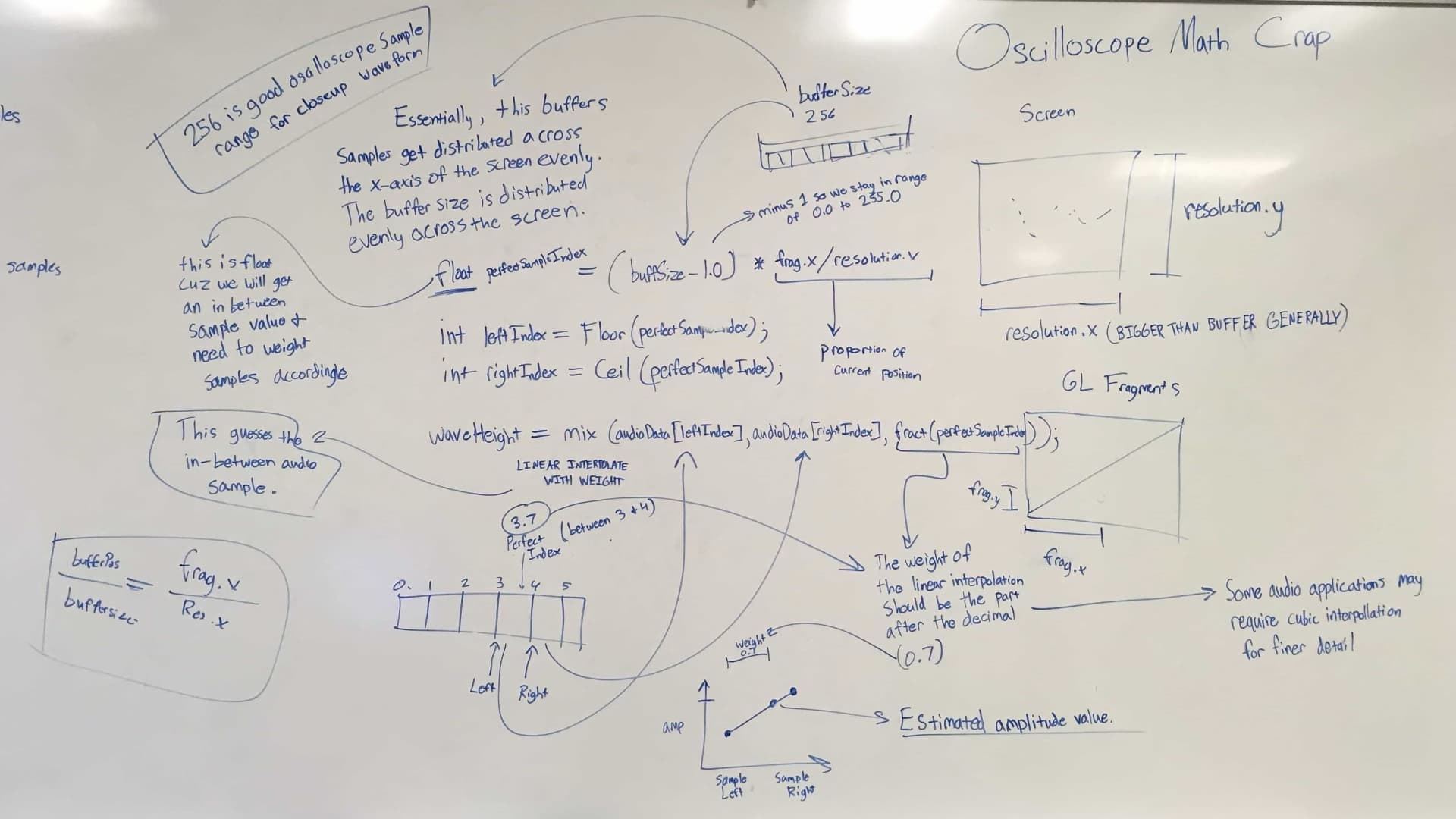
• Audio Waveform visualizations actually exclude a good amount of data. They tend to average the data because there is so much of it. For example, the most standard audio sampling rate is 44,100 samples per second. If you were to attempt to visualize all 44,100 samples in a single second of audio with one sample per pixel on your screen, it wouldn’t even fit on the screen! My Mac has a horizontal resolution of 2,880 pixels. That would only allow you to visualize 1/15th of all the audio stored in a single second! Various strategies are used to average this data and produce a good looking waveform. This blog post was very helpful. For my oscilloscope visualizations I used an interpolation technique instead of averaging samples together. I may write a post on this technique later.
• OpenGL and the GPU can handle a lot, including calculating and generating 3D points in realtime. In the 3D oscilloscope pipe visualizer I used the geometry shader to calculate many points on the fly on the GPU. The upside to this is less CPU processing is used to calculate points, allowing other threads to utilize more of the CPU. The downside is that it takes a bit of extra time to load this visualizer because it must instantiate a lot of variables on the GPU for processing. In this situation I probably would’ve just calculated the points on the CPU since it wouldn’t really have been that intensive to calculate.
• Dry-erase boards are helpful for understanding audio visualization algorithms.